Local contrast

A cluster_statistics feature, configured by LocalContrastFeature, that computes a per-emitter local-density contrast: each point's fine-scale kNN log-density minus the median fine-scale log-density over a larger surrounding neighborhood. Positive values mark points that are denser than their local background; the result is a per-emitter feature vector the caller thresholds directly.

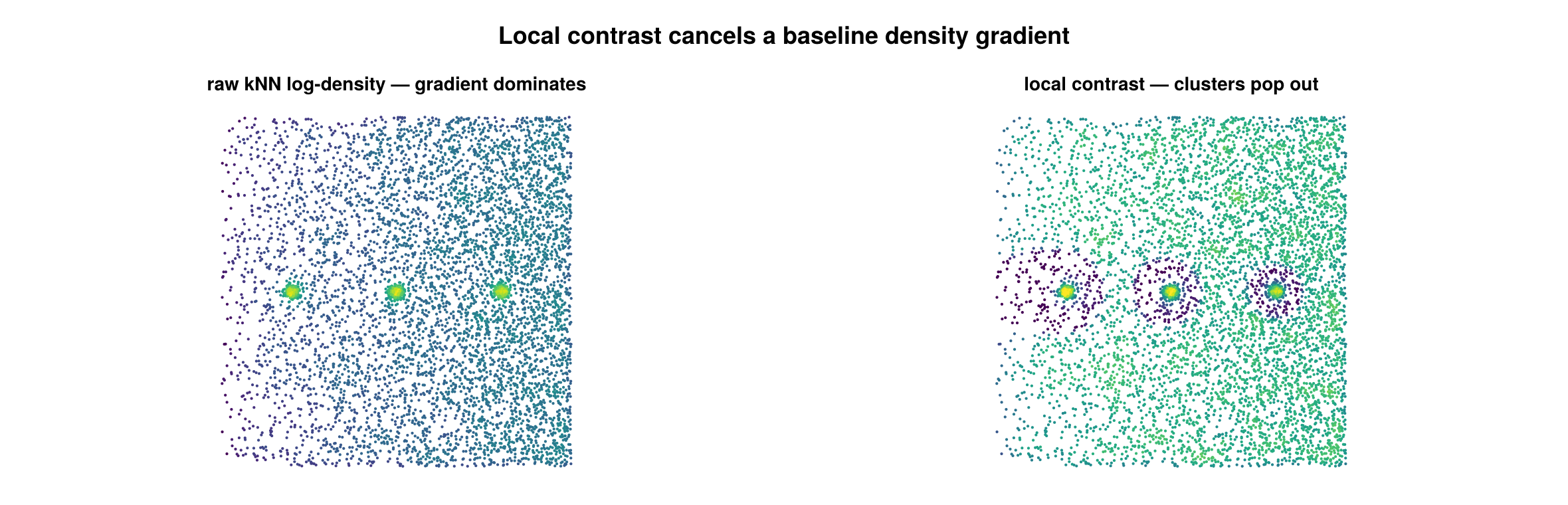
A baseline density gradient (sparse left → dense right) hides three clusters in the raw kNN density (left). Subtracting a local baseline cancels the gradient, so the clusters stand out (right).

Concept

A raw density estimate cannot tell a point in a compact structure apart from a point in a uniformly dense region — both report a high absolute density. Local contrast captures the elevation of a point's density above the density of its own surroundings: the same number of neighbors packed into a tight core gives a large contrast, while neighbors spread evenly over the baseline give a contrast near zero.

This matters because the absolute-density classifier (Otsu / GMM on log density) calls a point "structure" whenever its density exceeds a single global cutoff. When the baseline density varies across the field of view — cell-edge thinning, illumination falloff, a biological gradient — that one cutoff is wrong on at least one side of the cell. Subtracting a coarse local baseline cancels the gradient, so the feature fires only where a point is denser than its immediate neighborhood rather than denser than the cell-wide average. The per-emitter vector is meant to be thresholded into a foreground mask, e.g. as the seed/support gates of a point-hysteresis seed-and-grow on clouds with non-stationary baseline density.

How it works

Coordinates are taken in microns (µm) from the emitters (2D (x, y), or (x, y, z) when use_3d=true). A KDTree is built over the coordinate set (per dataset or pooled, see Configuration). Write $k_d$ for density_k and $k_b$ for background_k.

1. Fine kNN log-density. For each emitter $i$, let $r_{k}$ be the Euclidean distance to its $k_d$-th nearest neighbor (excluding the point itself). The kNN density estimate normalizes the neighbor count by the disk area $\pi r_k^2$, and the feature stores its natural log:

\[f_i = \log\!\left(\frac{k_d}{\pi\, r_{k}^{2}}\right)\]

The log keeps the downstream median and threshold comparisons on a comparable scale across a cell. If $r_k = 0$ (coincident coordinates), $f_i$ is set to NaN.

2. Local baseline. For each emitter $i$, take the median of $f_j$ over its $k_b$ nearest neighbors (excluding self, skipping any non-finite $f_j$). The median (rather than the mean) tolerates a small number of locally elevated neighbors without dragging the baseline up.

3. Contrast. The per-emitter feature is the difference

\[c_i = f_i - \operatorname{median}_{\,j \in k_b\text{-NN}(i)} f_j\]

Because it is a difference of logs, $c_i$ is the log-ratio of the point's fine density to its local baseline density: $c_i > 0$ means point $i$ is denser than its surroundings, $c_i \approx 0$ means it matches the baseline, and $c_i < 0$ means it is sparser. The value is reported in nats (natural-log scale).

Configuration

LocalContrastFeature is a Base.@kwdef struct <: AbstractStatisticsConfig:

Validation happens at the cluster_statistics call: background_k > density_k and density_k ≥ 1 are required, otherwise an ArgumentError is raised (the baseline must be coarser than the signal).

using SMLMClustering
using Statistics   # for `quantile` in the thresholding example below

# smld :: SMLMData.BasicSMLD
(_, info) = cluster_statistics(smld, LocalContrastFeature(density_k=200, background_k=2000))

info.statistic        # median of the finite per-emitter contrasts (scalar summary)
info.statistic_name   # :median_local_contrast
info.algorithm        # :local_contrast

contrast = info.extras[:contrast_per_emitter]      # Vector{Float64}, per emitter
fine     = info.extras[:log_density_per_emitter]   # Vector{Float64}, the fine f_i

# Threshold the per-emitter feature directly, e.g. seed/support gates for
# hysteresis seed-and-grow on a non-stationary baseline:
fine_floor = quantile(filter(isfinite, fine), 0.35)
seed    = isfinite.(contrast) .& (contrast .> 0.25)  .& (fine .> fine_floor)
support = isfinite.(contrast) .& (contrast .> -0.05) .& (fine .> fine_floor)
(smld_out, _) = cluster(smld, PointHysteresisConfig(graph_k=12, min_points=150);
                        seed=seed, support=support)

Output & interpretation

cluster_statistics returns (smld, info) where smld is the unmodified input (the statistics interface writes nothing onto the SMLD) and info is a ClusterStatisticsInfo:

• info.statistic — the median of the finite contrast values pooled across all groups; a single-scalar summary of the run. It is NaN when no group has enough points to compute the feature.
• info.statistic_name — :median_local_contrast.
• info.algorithm — :local_contrast.
• info.extras[:contrast_per_emitter] — Vector{Float64} of length n_locs_in, the per-emitter contrast $c_i$, in original emitter order. This is the primary output the caller thresholds.
• info.extras[:log_density_per_emitter] — Vector{Float64} of length n_locs_in, the fine kNN log-density $f_i$, also in original emitter order. Useful as a complementary absolute-density gate (e.g. require $f_i$ above a quantile floor in addition to a positive contrast).

Interpretation: a high positive contrast is a point sitting in a local density peak (a candidate structure point); a contrast near zero is a point whose density matches its surroundings (uniform background, regardless of how dense that background is); a negative contrast is a point sparser than its neighborhood. Because the baseline is local, the same contrast threshold applies on both the dense and the thin side of a density gradient.

Notes & caveats

• 2D / 3D. Both are supported via use_3d. The KDTree and neighbor distances are taken in the chosen dimensionality, but the density normalization is always the 2D disk area $\pi r_k^2$ in $f_i$ — even when use_3d=true. The contrast difference still behaves sensibly, but the absolute log_density_per_emitter scale is a 2D-area form, not a true 3D (volume) density.
• Too-small groups. A group with $n \le k_d$ emitters cannot be evaluated; those emitters receive NaN for both contrast and log-density (avoids a degenerate kNN query against a too-small set).
• background_k ≥ n in a group. $k_b$ is clamped to $n-1$ for that group, so the feature degrades gracefully to "log-density minus the group median," which is still well-defined.
• Coincident coordinates. A point whose $k_d$-th-neighbor distance is zero ($r_k = 0$) receives NaN log-density and NaN contrast. A point with no finite baseline neighbors also receives NaN contrast.
• per_dataset. When true, each dataset is built and evaluated on its own KDTree (no cross-dataset neighbors); when false, all emitters are pooled into one tree. Either way the per-emitter outputs are returned in original emitter order, and info.statistic is the median over the finite contrasts of the whole input.
• NaN handling. Both extras vectors are initialized to NaN and only filled where the feature is computable, so callers should mask with isfinite (as the example does) before thresholding or aggregating.